Quantum Computing for the Busy Developer – Part 1
A short introduction to quantum computing that compares it with well-known ideas such as GPUs and vectorization to show what it can and cannot do, and how custom optimization problems can be tackled with quantum technology.
Motivation
Quantum computers offer a particular kind of parallelism. Thanks to it, a quantum computer should be able to perform computations faster than a classical machine. To take advantage of this, however, problems have to be tackled in a different way, with algorithms designed specifically for it.
“Faster” here means that certain problems can genuinely be solved with a better computational complexity. In some cases the gap is dramatic: problems that take exponential time on a classical computer can be solved in polynomial time on a quantum one. (Well-known examples are the Deutsch-Jozsa algorithm and the famous Shor’s algorithm.)
These, however, are special problems that happen to fit the platform particularly well. As a developer, I want to find out whether more general kinds of problems can be solved this way too.
In this short series, I’ll show how to take a custom problem to a quantum computer and build a solution for it.
Plan
The series is split into four parts, each examining a quantum computer from a somewhat different perspective:
- Part 1 – gives a high-level picture of a quantum computer by comparing it with more familiar ideas such as GPU and vectorization.
- Part 2 – presents qubits and the other components behind that high-level picture.
- Part 3 – demonstrates what programming a quantum computer really looks like.
- Part 4 – walks through a working code example step by step.
A quantum computer at a glance
Example problem
To keep the discussion concrete, let’s concentrate on a single kind of problem – discrete optimization. We have a set of inputs and want to find the one that best meets some criteria (for instance the Travelling Salesman Problem – TSP for short – in which we look for the shortest route through all nodes of a given graph). Put more formally, we have a cost function and want to find its minimum.
Often this can be done with numerical methods, but only if the cost function meets certain requirements. In the general case, we essentially have to compute and compare the results for every possible argument.
Before going further, I want to introduce two extra assumptions:
- To keep things simple, we assume that the cost function both takes and returns single integers from a given range {0…N}. For problems with more complicated inputs, we can try encoding them as numbers (for TSP, say, by giving each route in the graph its own unique number).

A single-argument cost function
- We will turn the optimization problem into a decision problem. Suppose we don’t strictly need the very best result, just one that is good enough – that is, one meeting some predefined criteria (for TSP, any route shorter than a given limit might do). The cost function can then be replaced with a predicate that returns 1 for good inputs and 0 for all others.

A single-argument predicate
Thanks to the second assumption, we no longer have to compare results across inputs, which will come in handy when we try to parallelize the computation.
Now, with some luck, a single function call might already give us a good result. But if good results are rare, the expected number of calls will still scale with the total number of arguments.
Evaluating a function for every possible argument can soon become impractical – and this is where quantum computers could help.
Why use a quantum computer?
The optimization problem described above would force us to go through every possible result of the cost function. On a classical computer, this task has complexity O(n), where n is the total number of possible arguments. Note: we treat the function as a black-box here, and complexity is defined as proportional to how many times the function is called.
In Part 4, we will solve this example problem on a quantum computer with a quantum search algorithm, which brings the complexity of finding a solution down to O(√n). It isn’t an exponential speed-up, but it is still remarkable, and the approach is fairly general.
How can that be?
So what exactly is a quantum computer?
Put simply, a quantum computer is a machine that performs computation using quantum effects. These effects have one peculiar property – at times they act as though they were doing many things simultaneously. You might remember, for example, how an electron explores several paths at once in the double-slit experiment. Exploiting this property cleverly lets quantum computation run in parallel.
In some ways, this is similar to computing on a GPU.
The GPU as a coprocessor
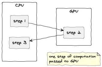
A GPU can act as a coprocessor for especially compute-intensive tasks. Machine Learning pipelines, for instance, often follow a pattern in which the heaviest parts of the computation are offloaded to the GPU.
The GPU as a coprocessor
Lighter tasks, such as preparing data and postprocessing, usually run outside the GPU. One can picture a similar setup in which certain well-defined tasks are handed off to a quantum computer, while data preparation and postprocessing take place on a classical one.
The analogy goes even further, though: computing on a quantum computer turns out to resemble vectorization.
Vectorization on a GPU
Computing in parallel with vectorization
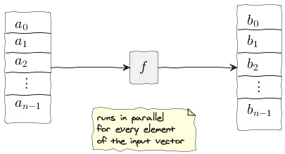
Vectorization is a technique for making efficient use of a GPU to parallelize computations. To apply it, our function typically has to be expressed with simple arithmetic operations and must avoid divergent branching.
We can then pass the function a single vector holding all the arguments, and the GPU parallelizes the work. Naturally, how many operations run in parallel is capped by the number of available cores.
Ideally, though, the entire computation can be expressed as a series of steps. In every step, all elements of the input vector are processed in parallel, and each step yields a new vector. Since every element is handled independently, the output vector has the same length. (Every element of the output vector matches one element of the input vector.)
Computing on a quantum computer looks somewhat like this.
Vectorization on a quantum computer
Computing in parallel on a quantum computer
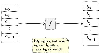
It is the same picture as before, except that n – the length of the vector – can reach 2ᵏ, where k is the number of qubits (qubits are discussed in more detail in Part 2).
Here, too, the function has to meet certain requirements. Some resemble those for GPU vectorization, while others are unique to quantum computers.
Most importantly, the function code must not branch – the computation has to apply the same set of operations to every argument. A function like that can process the entire vector of its arguments in parallel. What differs is that on a quantum computer the maximum number of arguments depends on the number of qubits, and every added qubit doubles that limit. This growth is exponential, so even with only a few qubits it soon exceeds the number of GPU cores.
At the same time, we must account for some extra, specific limitations:
- With GPU vectorization, vector elements could be any numbers. Here, with k qubits, the vector elements can only be unique binary integers of at most k digits.
- Unlike GPU vectorization, the length of the vector can change. This is possible because computations for the parallel inputs are not always independent of each other.
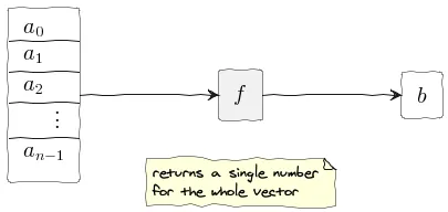
- Lastly, computing over the entire vector yields just one number.
Computing in parallel with one number as the result
Returning to our example
We will look more closely later at what these limitations mean and where they originate. For now, let’s quickly check whether they suit our example problem.
Our example cost function accepts inputs from a bounded set of integers {0…N}. We need enough qubits to represent every possible input (i.e., N < 2ᵏ). We will build a vector holding all the inputs and rely on the quantum computer’s ability to evaluate the function on all of them in parallel. We will also need some extra qubits to hold the intermediate results of the computation.
Example k bits of input plus some extra bits for intermediate results
Every input (an integer with k binary digits) gets some extra bits attached to it. In our case the input part stays fixed, while the extra bits change as the computation progresses. Together, the fixed part and the extra bits make up one vector element.
Each element can be thought of as a key-value pair, where the fixed part is the key and the rest is a mutable value. Because the key is unique and always there, every element stays unique for the entire computation.
In the end, we will make the quantum computer return the single input that meets the search criteria. To understand how, we have to dig a bit deeper – which is what comes next.
Summary
This part of the series offered a brief overview of a quantum computer. I compared it with more familiar ideas such as GPU and vectorization, pointing out both the similarities and the particular limitations a quantum computer imposes. I also outlined how a custom optimization problem could be brought to a quantum computer.
In Part 2, I’ll explain where these particular limitations come from, which means discussing qubits and the other building blocks of a quantum computer.
In Part 3 and Part 4, I’ll come back to the optimization example and examine it more closely, together with a working code example.