Quantum Computing for the Busy Developer – Part 3
This part of the busy developer's guide to Quantum Computing shows you what programming a quantum computer can really look like.
In the earlier Parts of this series, I briefly outlined what a quantum computer is and touched on qubits and the other building blocks underlying that picture.
This Part demonstrates what programming a quantum computer may look like in practice. (The examples and visuals below were created with IBM Qiskit, but they apply fairly universally.)
Programming a quantum computer
The earlier Parts explained what a computation on a quantum computer looks like. To recap: first we prepare a quantum register big enough to hold all of our inputs. We initialize it by placing it in a superposition – with the inputs represented by basic states. Next we apply a series of transformations – each one processing all inputs in parallel. Lastly, we perform a measurement and copy the result into classic memory.
Naturally, the transformations depend on the specific problem we are solving, so we need some way of defining custom transformations.
Not every transformation is allowed, however. In Part 1, while discussing vectorization, I pointed out that a quantum computer comes with certain constraints:
- a transaction cannot branch out – when applied to a register in superposition, it applies one and the same function to every basic state (every input),
- and the function has to be reversible.
Intuitively, “reversibility” means that every input maps to a unique output of the function, and vice-versa. Proving that a transformation is reversible is generally difficult without turning to algebra. Luckily, we can sidestep this problem by composing custom transformations out of existing ones.
Quantum gates
Complex transformations can be assembled from a palette of well-defined, simple operations known as gates. Many of these are similar to the logic gates found in a classic computer.
IBM Qiskit offers a palette of standard gates. This palette is universal – every other operation can be built out of these gates. And – since any combination of reversible operations is itself reversible – such custom operations are guaranteed to be correct.
A gate may be defined as a function over basic states. Below are a few single-qubit gates that I will use in the examples that follow.
Definitions of the I (Identity) and X (Not) gates
The I gate (Identity) does not change the qubit. I will later use it as a placeholder indicating that a qubit is left untransformed.
The X gate (logical Not) inverts the bit value of the qubit.
Phase, the concept introduced in Part 2, makes it possible to define further single-qubit operations that have no counterpart in a classic computer.
Definitions of the Z and Y gates
The Z gate flips the phase of the basic state |1⟩ and otherwise leaves the qubit as it is.
The Y gate combines Z and X.
Transforming a basic state may produce a superposition, which allows for even more gates.
Definition of the H gate (coefficient p stands for an evenly distributed probability)
The gate above is known as H (Hadamard’s gate). It is typically used to put a qubit into a superposition with evenly distributed probabilities.
Gates producing superpositions with other probabilities can exist as well. In fact, even a single qubit allows an infinite number of distinct gates.
Let’s also look at a definition of a gate that spans two qubits:
Definition of the CX gate (“control” on the left, “target” on the right)
This gate is known as CX (Controlled-Not). It can be understood as a conditional Not operation. The left qubit acts as the “control”, while the right qubit is the “target”. The input to the control qubit determines whether or not the target qubit gets flipped.
Quantum circuits
A set of quantum gates acting on qubits makes up a quantum circuit.
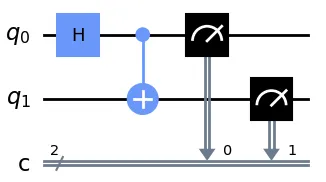
Example of a quantum circuit
Every horizontal line stands for a single qubit evolving over time. Gates act on the qubits one after another, changing their states. A gate may cover one qubit or span several.
This specific circuit places the qubits in an entangled state (coefficients left out for simplicity):
The entangled state produced
In this example:
- there are two qubits, q0 and q1, and two classic bits, c0 and c1 (the classic bits are collapsed)
- the H gate (shown here as a box with the letter “H”) acts on q0 only,
- the CX gate (shown here as a vertical line with a “plus”) spans q0 and q1,
- after that, q0 and q1 are both measured, and the results are copied to c0 and c1 respectively.
I will shortly explain in detail why this quantum circuit yields the entangled state. In the meantime, we can run an experiment to confirm that the resulting state really is entangled.
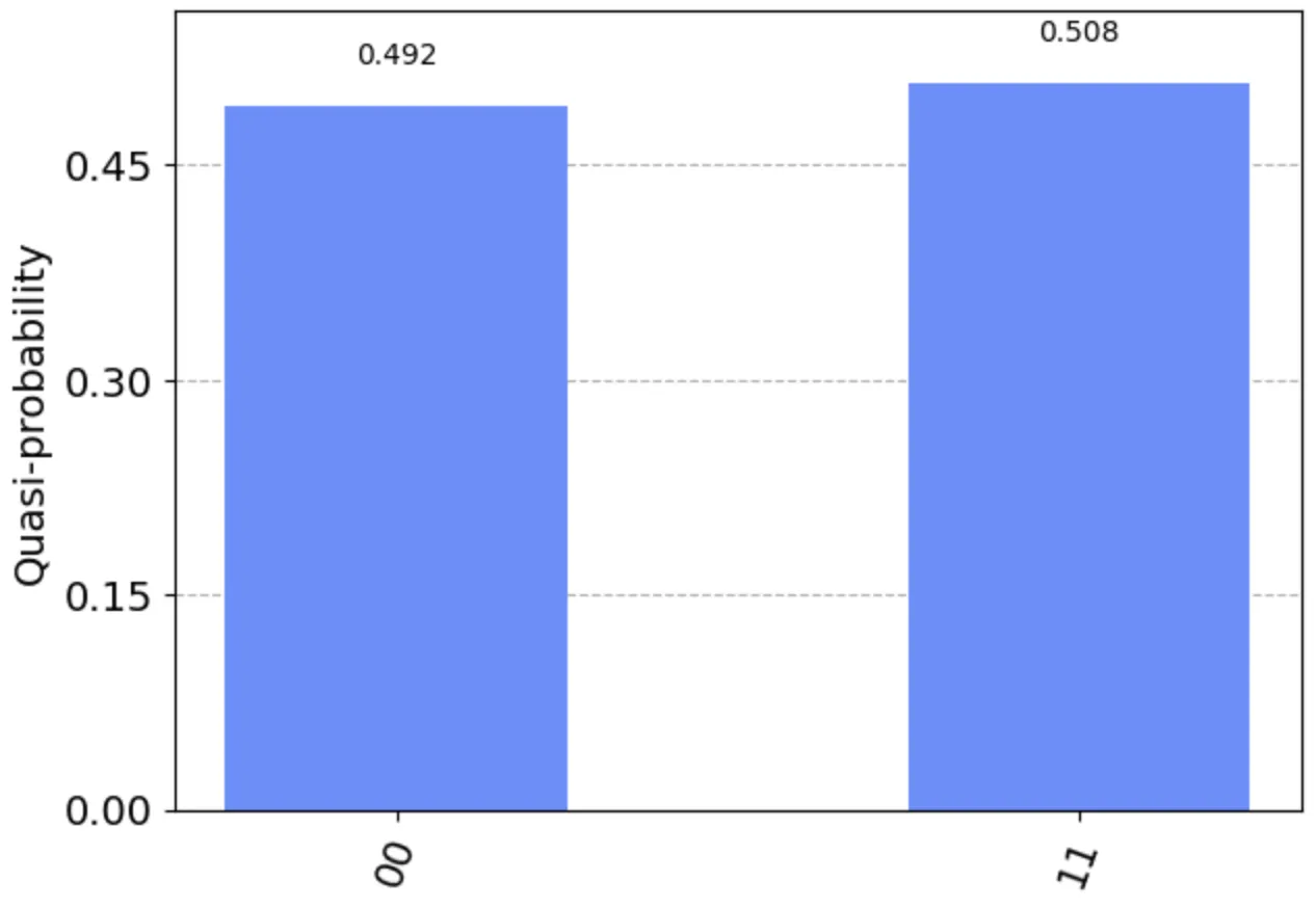
Outcome of an experiment running a quantum circuit with an H and a CX gate (2000 shots)
Let’s now analyze this circuit using the gate definitions presented earlier.
Analyzing a quantum circuit
Initially, qubits q0 and q1 are both set to |0⟩, so the starting state is |00⟩.
Next, the gates are applied one by one:
- Applying an H gate to qubit q0 produces a superposition: (|00⟩ + |10⟩).
- Applying a CX to |00⟩ leaves it unchanged: |00⟩.
- Applying a CX to |10⟩ flips the target qubit: |11⟩.
- Applying a CX to the entire superposition yields a superposition with the same probabilities, but with one basic state flipped: (|00⟩ + |11⟩). This is exactly the entangled state we expected.
In this circuit, the transformations of the individual basic states can be analyzed separately. That isn’t always possible, as the next example shows.
Transforming multiple states at once
For a simple example, consider a quantum circuit with a single qubit and two H gates:
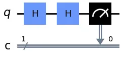
Example of a quantum circuit with two H gates
When the qubit starts at 0 and the gates are applied one after another:
- The first H gate turns the qubit state into (|0⟩ + |1⟩).
- The second H gate turns |0⟩ into (|0⟩ + |1⟩) and |1⟩ into (|0⟩ - |1⟩).
- Measured separately, these states would be impossible to tell apart. Combined in the resulting superposition, however, the two |1⟩s cancel out, so only |0⟩ remains as the result.
Running an experiment gives us:
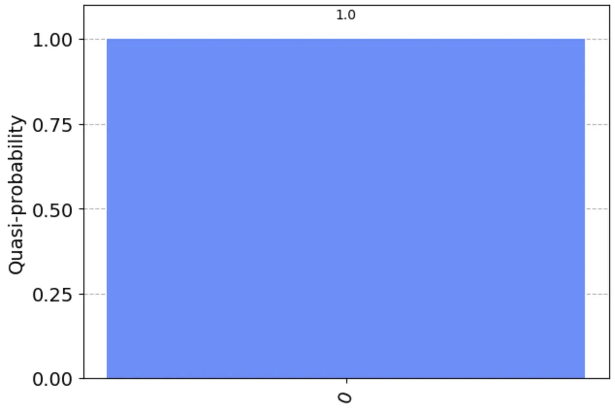
Outcome of an experiment running a quantum circuit with two H gates (qubit set to 0)
Likewise, when the qubit starts at 1:
- The first H gate turns the qubit state into (|0⟩ - |1⟩).
- The second H gate keeps the flipped phase of |1⟩ and turns |0⟩ into (|0⟩ + |1⟩) and ( -|1⟩) into (-(|0⟩ - |1⟩)), which simplifies to (-|0⟩ + |1⟩).
- Once again – measured separately – these states would be impossible to tell apart. Combined in the resulting superposition, though, the two |0⟩s cancel out, so only |1⟩ remains as the result.
Running an experiment this time gives us:
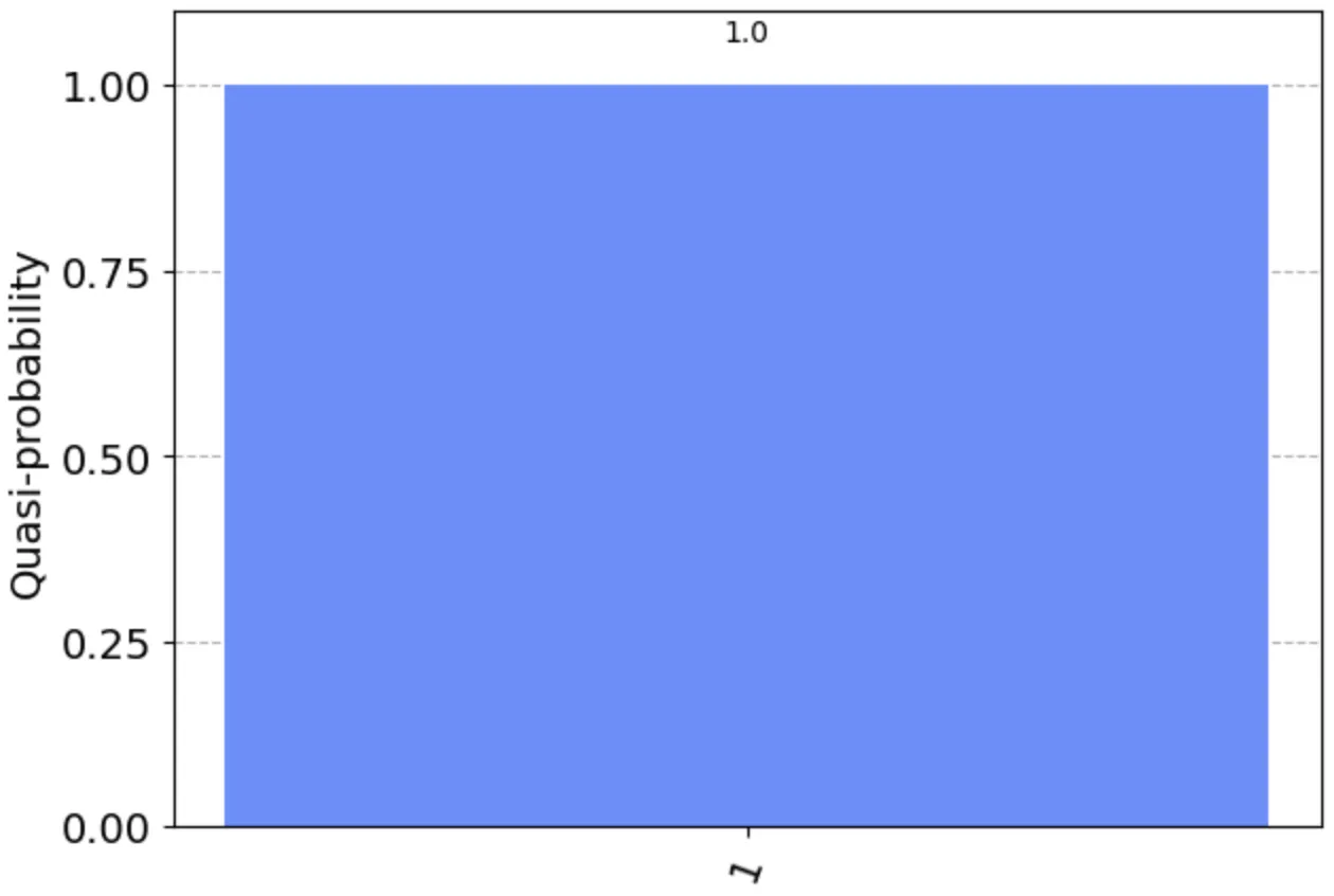
Outcome of an experiment running a quantum circuit with two H gates (qubit set to 1)
This example nicely illustrates how computing different basic states in parallel can make them influence each other in the result.
Before moving on to the running example, let’s quickly cover two more concepts.
Ancilla qubits
For another example, here is a quantum circuit containing a custom operation that spans every qubit.
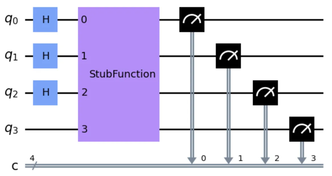
Example of a quantum circuit containing the StubFunction
In Part 4, we will use this operation as a test stub standing in for a search problem. The function checks whether a given input matches a hidden “password”. At this point, I want to draw particular attention to the role played by ancilla qubits.
The operation does not treat every qubit the same way. The first three qubits hold the actual inputs and are expected to be initialized with an H gate to every bitwise combination.
Example input bits plus one ancilla bit that stores an intermediate result
The fourth qubit is known as an ancilla. There can generally be more than one. It is set aside for storing intermediate results of the computation and is expected to start in the |0⟩ state.
In this example, the ancilla qubit becomes entangled with the input qubits during the computation. This lets the operation link every input with its own results, which is what makes parallel computation possible. I covered this in more depth in Part 2, in the section on entanglement.
In the end, the ancilla is disentangled and goes back to its initial state |0⟩.
Encoding information in gates
When you define an operation, keep in mind that not every piece of input information needs to be passed in through qubits. A large part of the problem will be encoded in its internal structure, in the form of gates.
For the StubFunction above, the structure of the gates encodes a hidden “password”.
For TSP, for instance, the input qubit values could serve merely to identify a specific route, while everything else needed to compute the route’s length could be encoded in gates.
Summary
This Part of the series introduced the ideas of quantum gates and circuits. I explained how gates can be combined into complex transformations, covered the role of ancilla qubits, and touched briefly on encoding information in gates.
Part 4 will bring all of these elements together in a running example.