Quantum Computing for the Busy Developer, Part 4
Quantum computing for the busy developer – a step-by-step tour of a working quantum search implementation.
In the previous Part of this series, I gave a short demonstration of what programming a quantum computer is like.
This Part presents a working example of quantum search (see: Grover’s algorithm). Below, I’ll take you briefly through its key points.
The implementation uses the IBM Qiskit Python SDK. Qiskit comes with a simulator that lets you try out the code on your local desktop.
A working quantum search example
Overall structure
The algorithm is built as a series of operations. They are defined from the bottom up, creating a nested structure.
Static predicate
The first of these operations is StaticPredicate.
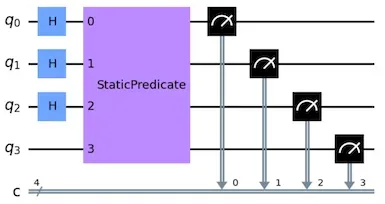
Sample quantum circuit containing the StaticPredicate
In essence, it is a test stub standing in for some search problem. It is statically set up with a binary sequence (a “password”) that specifies the input we want to find.
The qubits q0, q1 and q2 hold the inputs, while q3 is an ancilla qubit. (Ancilla qubits were covered in Part 3.) The input qubits are supposed to be in a superposition of every possible binary combination, and the ancilla qubit should start at 0. Each input is compared against the password, and for the chosen input the ancilla gets flipped to 1.
StaticPredicate is a composite operation. You can look inside it to examine its internal structure.
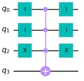
Internal structure of the StaticPredicate for the password “011”
The X (Not) and I (Identity; serving as a placeholder here) gates encode the “password”, and the MCX (Multi-Controlled-Not) gate flips the ancilla qubit.
Below is the outcome of an experiment that runs a quantum circuit containing only the StaticPredicate.
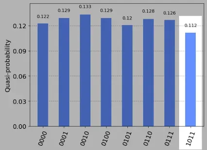
Outcome of a quantum circuit with the StaticPredicate (2000 shots; the chosen input is highlighted)
A side effect is that the ancilla qubit becomes entangled with the input qubits.
Stub function
The following operation is StubFunction.
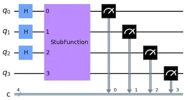
Sample quantum circuit containing the StubFunction
It wraps the StaticPredicate, but encodes the result in a different way – so that it meets the requirements of the Amplifier operation described below. The Amplifier needs the chosen input to be marked by a flipped phase. At the same time, it needs the ancilla qubit to be disentangled and set back to 0.
Below is the outcome of an experiment that runs a quantum circuit containing only the StubFunction.
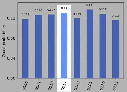
Outcome of a quantum circuit with the StubFunction (2000 shots; the chosen input is highlighted)
The ancilla qubit is flipped back to 0. The flipped phase does not show up in the result.
To produce the result, the StubFunction starts by applying a StaticPredicate. Next, it flips the phase of the chosen input with a Z gate. (Phase was discussed in Part 2, and the Z gate was defined in Part 3) Finally, it disentangles the ancilla qubit by applying the StaticPredicate in reverse. (This pattern is known as uncomputation.)
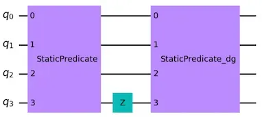
Internal structure of the StubFunction (the “dg” suffix marks an inverse)
Amplifier
The Amplifier operation implements the generic part of the quantum search algorithm. In essence, it raises somewhat the probability of every input marked with a flipped phase.
The Amplifier is a composite operation too. You can look inside it to examine its internal structure.
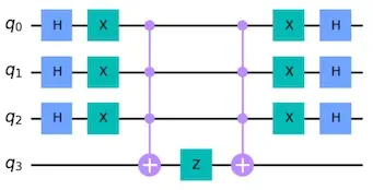
Internal structure of the Amplifier
The Amplifier is generic. It knows nothing about the “password” encoded in the StubFunction. (The exact gate structure comes from Quantum Computing by Nihal Mehta. How it works is explained clearly in Quantum Computing for Everyone by Chris Bernhardt.)
Below is the outcome of applying the Amplifier to the output of the StubFunction.
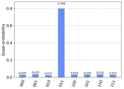
Outcome of applying the Amplifier to the output of the StubFunction!
The Amplifier operation can be applied a few times in a row. Every repetition raises the probability further. Incidentally, while doing this, it flips the phase back, and the mark on the chosen input is lost. That means that to keep amplifying the probability, the StubFunction has to be repeated too.
Search Iteration
Together, the StubFunction and the Amplifier make up one SearchIteration.
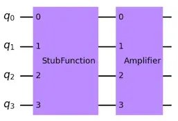
Internal structure of one SearchIteration
The SearchIteration has to be repeated a few times to maximize the probability of the chosen input.
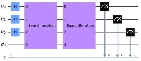
Quantum circuit with two search iterations
One can show that the highest achievable probability is reached after O(√n) iterations. Beyond that point, the probability begins to drop.
Below is the outcome of 2 iterations, the optimal number for 3 input qubits.
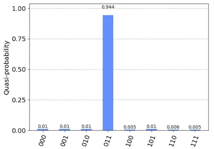
Outcome of 2 iterations for 3 input qubits (2000 shots)
Happy testing
I encourage you to experiment with the sample project. For instance, the code makes it simple to raise the number of input qubits.
As an example, below is the outcome of 724 iterations for 20 input qubits.
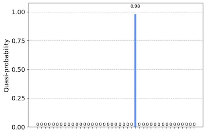
Outcome of 724 iterations for 20 input qubits (2000 shots)
With this many iterations, the probability of finding the “password” gets close to 0.98. Keep in mind that a classical computer would need 10⁶ iterations to locate the chosen input with the same probability.
Summary
This Part took you through a working implementation of quantum search. I built the solution out of two complex gates:
- the StubFunction – standing in for a custom search problem,
- the Amplifier – a generic implementation of Grover’s algorithm.
By swapping the StubFunction for any cost function that meets the basic assumptions laid out in Part 1, you obtain a generic scheme for tackling a broad range of optimization problems on a quantum computer.
Where to go next
Today, there are plenty of excellent resources for getting started with quantum computing. Since the field began, much work has gone into making it easier to approach.
If you like a clear theoretical foundation, I strongly recommend Quantum Computing for Everyone by Chris Bernhardt. If you lean towards a more practical approach, take a look at Quantum Computing by Nihal Mehta.
The IBM Qiskit website is another excellent source of learning materials.