Quantum Computing for the Busy Developer - Part 2
This Part covers qubits and the other building blocks of quantum computing.
Introduction
This Part takes a closer look at qubits and the other building blocks of a quantum computer.
I’ll keep things light and cover only what you need to follow the reasoning in this discussion.
We begin with a single qubit.
Single qubit
The qubit is the fundamental building block of a quantum computer. It stands for one quantum effect. Well-known examples of such effects are the energy levels of a trapped ion, photon polarization and electron spin.
A qubit can be seen as an abstraction that conceals the physical implementation (a two-level quantum mechanical system) and reveals only the properties that matter for quantum computation.
A qubit can switch between two states – we can label them 0 and 1. In that respect, a qubit is similar to a single bit of classical computer memory. Sometimes, however, a qubit behaves as if it were in both states simultaneously. Such a qubit is said to be in a superposition.
There are two kinds of operations we can perform on a qubit: transformation and measurement.
Measuring a qubit
We cannot simply look inside a qubit to find out its state. To read the value of a qubit, we first have to measure it. Only after that can we copy the value into classical memory and use it further.
A measurement always yields a definite value: 0 or 1 – whether or not the qubit was in a superposition. Measuring a qubit that is in a superposition forces it to pick one of the two values. The outcome of such a measurement is random – we cannot tell in advance which value a given qubit will return, but we can predict the probability of obtaining each value when measuring.
Moreover, a measurement resets the state of the qubit. A second measurement made right after the first will always give the same value. This means that measuring a single qubit does not tell us whether it was in a superposition. To reconstruct information about the superposition, we have to run an experiment on a series of qubits prepared in the same way. In Part 3, you’ll see how to run such experiments in IBM Qiskit.
In such an experiment, we take a large number of identically prepared qubits and measure them one after another to collect statistics. The statistics are random, but they should match the predicted probability.
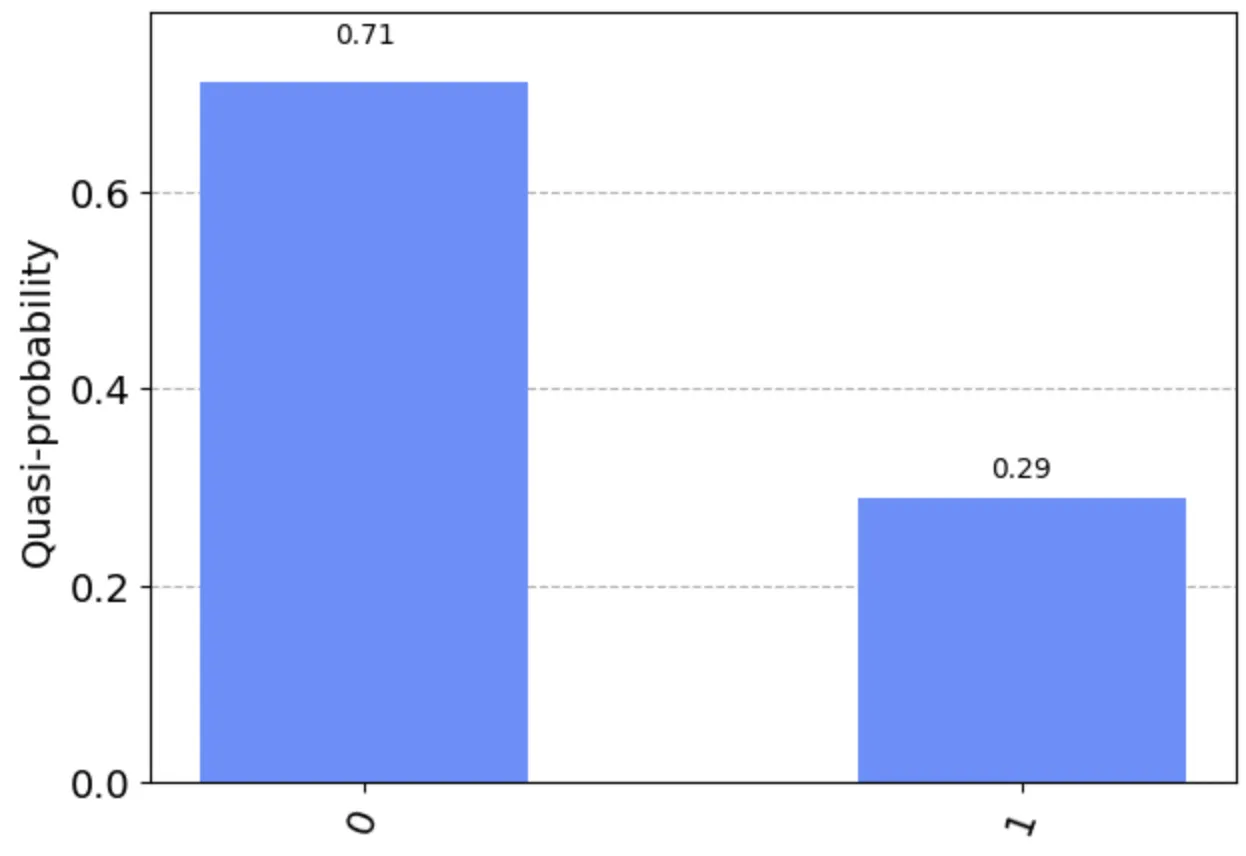
The outcome of an experiment with a single qubit in a superposition whose probability is unevenly distributed
The basic qubit states are typically written as the symbols |0⟩ and |1⟩. A superposition is written as a linear combination of the basic states:
A superposition with arbitrary probabilities
The coefficients a₀ and a₁ stand for the probability of obtaining each value when measuring. To keep things simple, I’ll mostly leave these coefficients out from now on. In what follows, a combination written without coefficients denotes a superposition with evenly distributed probabilities:
A superposition with evenly distributed probabilities
Transforming a qubit
A transformation lets us change the state of a qubit without measuring it. Every transformation can be defined as a function on the basic states.
A sample transformation defined on the basic states
The transformation shown above, for example:
- turns a qubit in state |0⟩ into |1⟩ when applied to it,
- turns a qubit in state |1⟩ into |0⟩ when applied to it.
This transformation is similar to the logical Not operation in a classical computer. You can think of it as a logical operation that flips the qubit’s bit value. In Part 3, I’ll say more about how to define your own transformations.
The key point is that a transformation works without any measurement. When it is applied to a superposition, the transformation acts as if it were processing both basic states in parallel, and the probabilities are preserved.
Suppose, for example, that a qubit is in a superposition where the probability of measuring |0⟩ is 0.75 and the probability of measuring |1⟩ is 0.25. Applying the transformation above to this qubit keeps the probabilities but flips the bit value of both basic states. Afterwards, the probability of measuring |0⟩ is 0.25, and the probability of measuring |1⟩ is 0.75.
Notice that nothing here is random, even though we are talking about probabilities. Randomness only comes in when measuring the qubit forces it to pick one of the two values.
That brings us back to vectorization.
Qubit and vectorization
A transformation on a qubit can be viewed as the simplest form of vectorization.
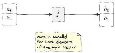
One qubit as the simplest form of vectorization
Here, the function stands for a transformation that operates on both vector elements in parallel. The vector consists of two elements, corresponding to 0 and 1. Each element stands for the expected probability of obtaining that value when measuring.
Qubit transformations have one more particular property that can feel counterintuitive. The result of a transformation on one element can affect the probability of the other element, and the other way round. Several results computed in parallel can reinforce a given probability or cancel one another out.
To see how probabilities can cancel out, we need to say a few words about phase.
Probability and phase
In quantum computing, a probability is described by two parameters: amplitude and phase. In this respect, it behaves somewhat like waves. I’ll use a simplified description here and assume that phase can only be the same or opposite (see: Quantum Computing for Everyone by Chris Bernhardt).
Remember that when two identical waves meet crest-to-crest, they reinforce each other – we say they are in the same phase. When they meet crest-to-trough, they cancel each other out – we say they are in opposite phases.
We will mark an opposite phase with a “minus” sign placed in front of a basic state or a superposition. In the superposition below, for example, the “minus” sign indicates that the basic states |0⟩ and |1⟩ are in opposite phases:
A superposition whose probabilities are in opposite phases
Phase does not affect measurement. The actual probability of obtaining a given value when measuring is determined by the amplitude alone. During computation, however, phase is very important. It lets us cancel out undesired results of the parallel computation.
Quantum register
Qubits arranged together in a sequence form a quantum register. Let’s see how the rules that apply to single qubits extend to the entire register.
Rather than looking at the separate states of individual qubits, we will look at the joint state of the entire register. With two qubits, for instance, the register has these basic states: |00⟩, |01⟩, |10⟩, |11⟩. Each basic state is written here as |ab⟩, where “a” and “b” stand for the states of the individual qubits in the register – the left bit is the state of the first qubit, and the right bit is the state of the second one.
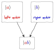
A basic register state as a combination of qubit states
Every basic state of a register of length k maps to one binary integer of that length – each qubit stands for one binary digit.
A quantum register, just like a single qubit, can be in a superposition. And, just like a single qubit, it can be transformed and measured.
Measuring a register
To measure a register, we measure its individual qubits one after another. The qubits can be measured in any order.
Every measurement of an individual qubit yields a definite value: 0 or 1 – corresponding to one digit of a binary integer. Getting the full integer requires measuring every qubit.
A register in a superposition behaves as if it were in many basic states simultaneously. Once more, we cannot tell which value a particular set of qubits will return, but we can predict the probability of obtaining given values when measuring.
Generally, a superposition of the register can be written as a linear combination of basic states with coefficients standing for probabilities:
A quantum register in a superposition with arbitrary probabilities
As before, for a superposition with evenly distributed probabilities, I leave these coefficients out to keep things simple:
A quantum register in a superposition with evenly distributed probabilities
Entanglement
In some cases, a superposition can be split into independent states of the individual qubits:
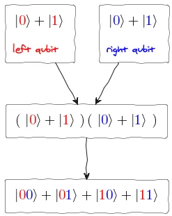
A quantum register state composed of the states of two qubits in superpositions
The superposition above is a linear combination of two qubits, each in a superposition. Combining every basic state of the left qubit with every basic state of the right qubit yields the resulting state of the register.
Here, the expected probabilities of measuring each qubit stay independent. Measuring one qubit – whatever the result – does not change what we expect from measuring the other qubit.
The state of a register, however, is not always just a combination of the states of its individual qubits. A register can be in states where the expected probabilities of individual qubits depend on one another. Such qubits are called entangled.
Take, for example, this register state:
A quantum register in an entangled state
Here, if measuring one qubit gives 0, measuring the other qubit will always give 0 as well. Likewise, if measuring one qubit gives 1, measuring the other qubit will always give 1. It does not matter which of the qubits is measured first.
Role of entanglement
Quantum entanglement is a necessary ingredient of the quantum computational speed-up in many algorithms (see: Jozsa-Linden). It is also central to the approach to solving custom problems that I present in this series.
Entanglement is what lets us build the key-value pairs.
A key-value pair: k bits for the key plus extra bits holding the value
The figure above shows a single basic state of a register made of many qubits. The first _k _qubits hold a fixed key, and the remaining qubits hold a changeable value linked to that key.
Usually, though, we don’t want to keep just one key-value pair in the register. Instead, we want a superposition that represents many key-value pairs at the same time. Entanglement makes this possible.
To achieve it, we create a superposition that contains every key and entangle each key with its corresponding value. Entanglement lets us link any value to any key within the superposition.
Transforming a register
A transformation on a register can cover several qubits at once. For instance, to be able to create entangled states, a transformation has to cover at least two qubits. I’ll go into this in more detail in Part 3.
Just as before, a transformation applied to a superposition behaves as if it were processing all basic states in parallel, keeping their probabilities.
Just as before, the result of transforming one element can affect the probabilities of the others. Several results computed in parallel can reinforce a given probability or cancel one another out.
Register and vectorization
Following the same reasoning, a transformation of the register can be viewed as a kind of vectorization.
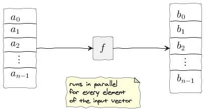
A transformation that processes all basic states in parallel
Here, the function stands for a transformation that operates on all vector elements in parallel. The elements of the vector correspond to all basic states of the register. Each element stands for the expected probability of obtaining a given value when measuring.
Measuring every qubit in the register produces one value – one binary integer of length
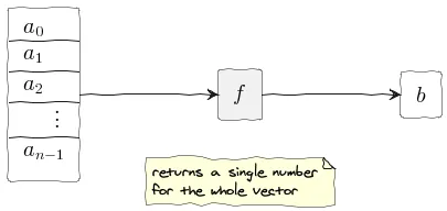
Measuring every qubit produces one value
Putting it all together
As a result, we are back at the following picture:
- In this case, a vector stands for the state of a quantum register – which may be in a superposition.
- Every vector element maps to one binary integer and stands for the probability of obtaining that value when measuring.
- The computation is a series of transformations applied to the register. Every transformation yields a new vector.
- At the end, a measurement produces one number. The outcome may be random, but its probability is set by the transformations that came before.
- The trick lies in steering the computation so that the probability of obtaining the expected result when measuring goes up.
Summary
This Part briefly covered qubits and quantum registers. I described the two kinds of operations that can be performed on them: measurement and transformations. I explained superpositions and how they relate to measurement and transformations. I touched on specifically quantum properties such as probability phase and quantum entanglement. I showed how all these ideas connect to the vectorization analogy introduced earlier.