Does Vibe Coding Work for Machine Learning?
Could vibe coding transform ML workflows? We put the Cursor coding agent to the test in EDA, modeling, explainability, and deployment to see.
Vibe coding has caught on so quickly that it already has a Wikipedia page of its own. In case you haven’t heard of it yet, vibe coding is a new development technique in which code is written and applications are built using natural language. It has already shown strong results in several areas of software development. Machine Learning (ML) covers a broad set of tasks, such as:
- visualizing data,
- training models,
- evaluating them,
- deploying them.
Coding agents can obviously speed up routine programming work, but the more important question is whether they can genuinely support the core ML workflows.
In this article I’ll use Cursor as the agentic code editor. I’ve also tried coding agents in VSCode, but in my experience Cursor offers a smoother and more efficient workflow, especially for ML-related development.
Datasets
For my tests I picked two very different datasets: the plant-disease dataset from DiaMOS and the Unemployment Duration dataset. Their structure and complexity differ considerably, which let me check how well coding agents cope with both simple and more demanding ML problems.
The plant-disease dataset poses a fairly simple supervised learning task: a 4-class classification problem. Every image shows a kind of plant leaf and carries one of four disease labels. That makes it a good fit for testing basic training pipelines, image preprocessing, and explainability techniques like Grad-CAM or saliency maps. The classes are moderately imbalanced, but on the whole the dataset is clean and visually consistent, which allows quick prototyping and model iteration.
The Unemployment Duration dataset, on the other hand, is a much harder challenge. It is a survival analysis problem: the target isn’t a fixed label but the length of unemployment, accompanied by censoring indicators that tell whether the event (getting a job) happened. The dataset contains several one-hot encoded variables, numeric features (e.g., age, wage), and temporal components. Such a structure calls for a deeper grasp of what each variable means – above all the censoring logic – so that analysis and modeling don’t yield misleading results.
The two datasets complement each other: one is about efficiently classifying image data, the other about the subtleties of censored time-to-event prediction. Together they provide a solid basis for assessing what agent-driven machine learning workflows can and cannot do.
Exploratory Data Analysis
The prompt for exploratory data analysis (EDA) was very simple:
Create EDA for plant-disease from scratch as a jupyter notebook.
To get the output written straight into a notebook, I needed to use the Sonnet-4 model.
The resulting notebook was impressive. Apart from a few small plot alignment problems, it delivered a helpful set of basic EDA outputs: visualizations for every class, class distribution statistics, plus image size ratios and frequency distributions. The analysis made it obvious right away that the dataset was imbalanced.
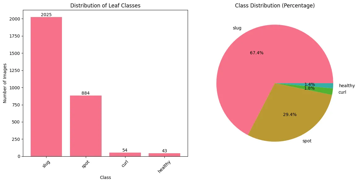
The model also offered practical suggestions derived from what it found, aimed at boosting model performance by tackling possible problems in the dataset.
This approach considerably accelerates the early EDA stage, since code and results tailored to the dataset are generated automatically. ML practitioners still need to check the outputs, though. Image datasets are well suited to this sort of automated analysis, but more complex data structures can result in wrong conclusions or faulty visualizations.
Potential Issues:
- Class imbalance was found. The model proposed handling it with data augmentation or a weighted loss function.
- Image sizes were fairly uniform, which makes preprocessing simpler.
Recommendations:
- Use data augmentation to enlarge the dataset and improve generalization.
- Split train/validation in a stratified way so the class distribution is preserved.
- Resize every image to the same dimensions (e.g., 224×224) to standardize the input.
- Normalize images with ImageNet statistics, particularly when using transfer learning.
Potential problems
The unemployment dataset provides a good example of an EDA result that isn’t entirely correct. Below is a summary of what the model produced in two iterations on the same dataset.
Cursor’s output
First iteration:
🔍 KEY FINDINGS:
- UI recipients: 8.0 weeks average
- Non-UI recipients: 4.1 weeks average
- Difference: 3.9 weeks (longer for UI recipients)
Second iteration:
⏱️ DURATION INSIGHTS:
- Average duration: 6.2 weeks
- Median duration: 5.0 weeks
- Duration variability: 5.6 weeks (std)
- Range: 1-28 weeks
- Distribution: Right-skewed (skewness = 1.52)
🔍 KEY FINDINGS:
- UI effect: +3.9 weeks (longer for UI recipients)
- Age correlation: 0.153 (positive relationship)
- Wage correlation: 0.040 (higher wages = longer search)
- Replacement rate correlation: -0.030
Clearly, the results differ from run to run, even though the dataset hasn’t changed and the results come from code the model itself generated. Worse still, neither output is correct.
The root of the problem lies in the dataset’s structure, which contains four one-hot encoded censoring variables describing how the unemployment spell ended.
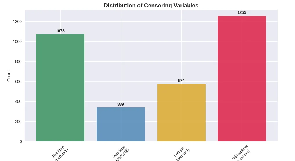
These variables tell us what kind of event ended (or did not end) the unemployment period. Sadly, the model handles them as independent input features instead of outcome-related indicators, even though the accompanying documentation spells out their purpose clearly.
For example, when the recorded duration is 14 weeks and censor4 equals 1, the subject was still unemployed when the observation window closed, and the event (getting a job) never took place. The real duration is then right-censored – the unemployment spell lasts longer than the 14 weeks captured in the dataset.
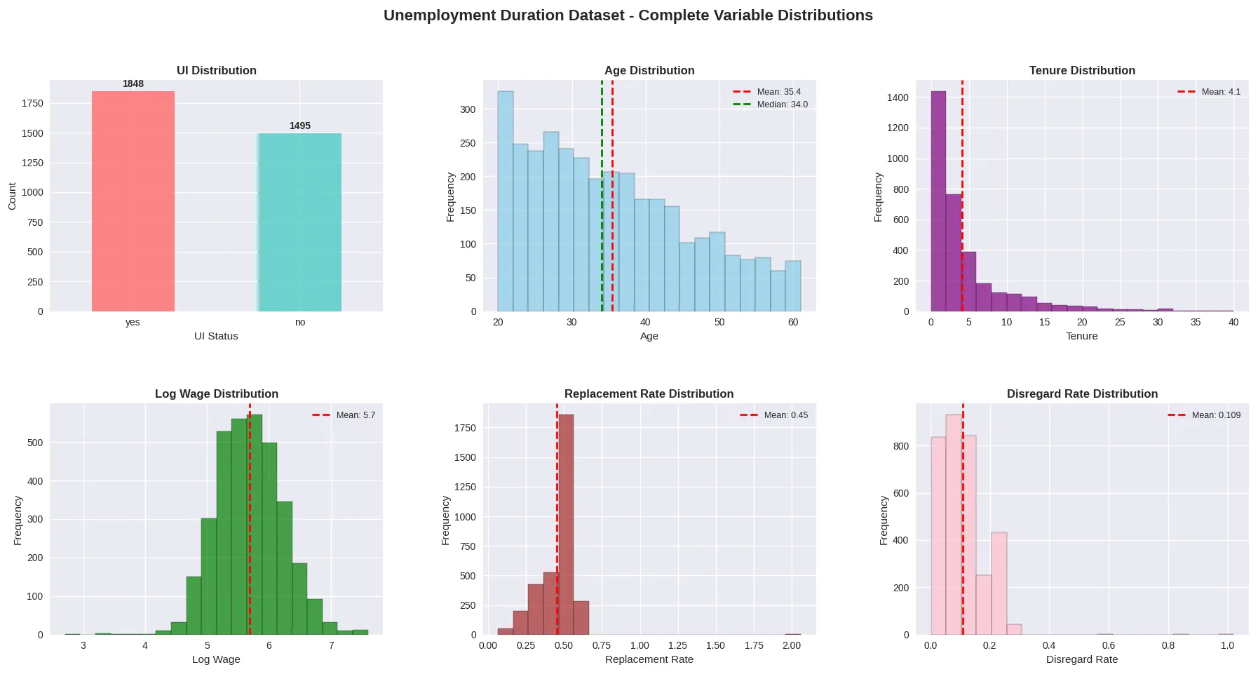
The dataset’s explanatory variables are listed below:
AutoML vs Vibe Coding
Many of today’s AutoML frameworks let you build complete machine learning pipelines with little manual effort and only modest ML knowledge. This greatly lowers the barrier to entry, but it frequently produces black-box models with little flexibility, which makes debugging, extending or interpreting the results harder – particularly in complex or regulated settings.
Vibe coding, by contrast, uses natural language prompts and large language models to support developers who already have machine learning expertise, or who can at least check and validate the results. It can accelerate building ML pipelines while keeping full control over the code, the architecture and interpretability. Developers are free to extend or adjust the pipeline as needed, finding a balance between automation and transparency. The table below gives a high-level comparison of the two approaches:
| Aspect | AutoML | Vibe Coding |
|---|---|---|
| Goal | Automates the whole ML pipeline end to end | Produces ML code from natural language prompts |
| Flexibility | Low–medium; fixed, predefined workflows | High; fits any coding scenario |
| Ease of Use | Very easy; hardly any coding needed | Needs coding skills and an understanding of ML |
| Best For | Quick prototyping, structured data, business applications | Custom ML workflows, experiments, PoCs |
| Learning Value | Low; hides most of the complexity | High; promotes hands-on ML learning and iteration |
Vibe coding PoC image classificator
In my tests I relied on automatic model selection and started with this prompt:
Build a lightweight image classification model in PyTorch to classify leaf images into 4 categories. Use one of small image classification models. Load images from a directory, and include preprocessing, training, and evaluation steps. Keep the code modular, efficient, and well-commented.
On the plant-disease dataset, Cursor produced code covering data loading, basic preprocessing, a train-validation split (albeit without a fixed random seed), model training and evaluation. The reported training accuracy hit 87% – which sounds impressive at first, doesn’t it?
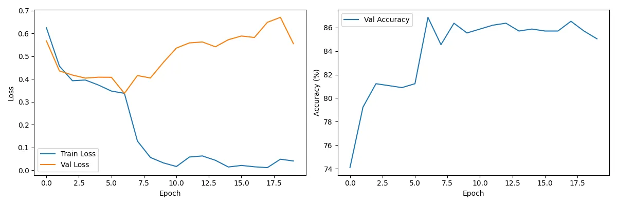
The plots present loss metrics on the transformed dataset
There are, however, several problems worth pointing out:
- Overfitting risk: The loss plots show training and validation losses drifting apart from some point on, a sign that the model begins to overfit. Training probably should have ended sooner.
- Wasted computation: Many of the training epochs most likely brought no extra performance and could have been skipped to save time and resources.
- Unseeded split: Because the dataset split had no seed, results can’t be reliably reproduced and the trained model can’t be properly tested, as we don’t know which data ended up in which set.
- Metric limitations: An accuracy of 87% may look impressive, but in a 4-class classification problem it can be deceptive, particularly with an imbalanced class distribution. Without insight into the class proportions, the model may simply have learned to predict the dominant class, which could make up 87% of the samples. Accuracy on its own isn’t enough in such a case. More informative metrics include the F1 score, ROC curves (per class), or a complete classification report giving precision, recall and support for every class.
After several iterations I managed to add early stopping with a patience of 3 epochs and set up training to save the best-performing model. The agent could not make these changes by itself and needed manual guidance to get them right.
Thanks to these improvements the model did well on the test set, reaching an accuracy of 0.867 and an F1 score of 0.869.
Here is the full classification report:
            precision    recall  f1-score   support

     healthy     0.7500    0.8571    0.8000         7
        spot     0.7634    0.8680    0.8124       197
        slug     0.9307    0.8660    0.8972       388
        curl     1.0000    0.9000    0.9474        10

    accuracy                         0.8671       602
   macro avg     0.8610    0.8728    0.8642       602
weighted avg     0.8750    0.8671    0.8691       602
On the plus side, Cursor did a great job building the DataLoader, including proper normalization with MobileNet’s ImageNet statistics during preprocessing. All in all, the experiment showed that this type of classification is feasible, and Cursor quickly put together a PoC that more or less worked.
AutoML PoC
I also checked how the results of a vibe-coded solution stack up against an AutoML approach. For the comparison I used AutoKeras, which builds image classification models automatically from a set of pretrained architectures like EfficientNet, ResNet, Xception, and MobileNet.
I set AutoKeras to run 5 trials, and its best model reached 67% accuracy. That number is deceptive, however. The AutoML process seemed overly fixated on minimizing validation loss, so it settled on a model that just predicted the majority class. Accuracy means little here, since the model learned to assign almost every sample to one dominant class.
Curiously, AutoKeras concluded that none of the pretrained architectures on offer were a good fit and chose to train a vanilla CNN from scratch instead. The classification report below summarizes how this model performed:
             precision    recall  f1-score   support

           0       0.00      0.00      0.00         8
           1       0.00      0.00      0.00         7
           2       0.67      1.00      0.81       304
           3       0.00      0.00      0.00       132

    accuracy                           0.67       451
   macro avg       0.17      0.25      0.20       451
weighted avg       0.45      0.67      0.54       451
This output makes the class imbalance issue and the model’s inability to generalize across all classes plain to see. Although the accuracy looks reasonable on the surface, the macro F1 score and per-class metrics expose large performance gaps.
Apart from the limitations and errors I ran into, the process wasn’t entirely simple either. The dataset was big enough that cloud-based AutoML tools were impractical because of upload and processing limits. On top of that, AutoKeras doesn’t take care of data loading, so I had to write my own data loader, apply the required preprocessing, and split the dataset into training, validation and test sets by hand.
Experiments
Next, I went back to the plant-disease dataset and used this prompt:
Create experiments for leaves model.
The code the agent proposed was adequate for basic validation and contained three tiers of experiments meant to test different configurations of the training pipeline. They were structured like this:
- Simple Experiments checked combinations of three learning rates, three batch sizes and three optimizers.
- Quick Experiments went further, covering a wider range of hyperparameter combinations and adding data augmentation techniques.
- Full Grid Search ran an exhaustive sweep over every possible combination of the defined learning rates, batch sizes and optimizers.
This is a good starting point for early experimentation. Every experiment type runs for a single epoch, and the code works properly, reporting accuracy metrics for the various parameter configurations. It also does basic logging of the parameters used in each test.
Here are the results of the simple experiments:
🎯 Best Learning Rate: 0.001 (81.73%)
📦 Best Batch Size: 32 (83.89%)
⚡ Best Optimizer: SGD (84.72%)
What’s missing, though, is dataset version tracking, and it depends entirely on grid search. Even with the option to cap the number of tests, it remains lacking in efficiency and flexibility.
Random search or deterministic samplers such as TPE are a more efficient alternative to grid search, as they optimize results without exhaustively trying every combination. Tools such as Hydra together with the Optuna Sweeper make experiment management even simpler and allow advanced, parallelized hyperparameter tuning.
Explainability
I tried out explainability on an NLP-based classification model by adding SHAP to examine feature impact. The agent, however, didn’t fully understand the pipeline. It used sample text inputs unrelated to the real dataset and even produced examples in the wrong language. After several attempts, it still couldn’t deliver a meaningful result. More precise and detailed prompting might have made it work, but I think writing such a specialized prompt takes more time than implementing explainability by hand.
Turning back to the plant-disease dataset, I wanted to assess the explainability of the image classification model generated earlier. I asked the agent for Feature Activation Maps, Grad-CAM, and Saliency Maps.
The results worked, but getting there was inefficient. The agent wrote more than 1,000 lines of code scattered over several versions of near-identical scripts (e.g., grad_cam.py, simple_grad_cam.py, working_gradcam.py, etc.), and the whole thing took about 30 minutes. In practice, these visualizations could have been done in fewer than 50 lines of compact, readable code. The final output was technically correct, but the agent’s overhead diminished its real-world usefulness.
Deployment
In another test, I asked Cursor to help deploy a more complex machine learning pipeline.
The pipeline being evaluated consisted of several parts. First, PaddleOCR scanned receipts and converted them into line-by-line text. Next, product descriptions were tokenized with the all-MiniLM-L6-v2 sentence transformer. Lastly, the embeddings went into an XGBoost classifier that assigned one of six predefined product categories.
Cursor couldn’t produce a fully working solution without heavy manual intervention. It picked the wrong models (the original version rather than a locally fine-tuned one), used different OCR configurations, and displayed results inconsistently from one iteration to the next. Getting a working implementation took a step-by-step dialogue with refined prompts and manual fixes to various components.
In the end, after several iterations, the pipeline was deployed successfully. It used FastAPI to serve the model and Gunicorn as the application server. Cursor also built a simple user interface for uploading images and viewing the output. The setup was nowhere near production-ready, but it made a solid proof-of-concept and showed that the approach is viable.
One could argue about this, but Cursor appeared to lose its way a number of times while debugging. In some situations, writing the code by hand – or rather with chat – might have led to a working solution faster, largely because the solution could be shorter than a detailed prompt. The large context and complexity of the pipeline were probably to blame. One clear plus, however, was the generated visual presentation of the results, which looked clean and intuitive.
Conclusions
Coding agents are without doubt a central part of programming’s future. Yet experienced machine learning practitioners are still indispensable for overseeing and steering development. In the hands of someone with domain expertise, these tools bring clear productivity gains. They can, however, easily yield misleading or incorrect results when used by people without a solid grasp of the underlying methods.
In practice, coding agents act more like next-generation IDEs – they shine when autocompleting supervised code or producing well-defined functions from precise, expert-level instructions.
Coding agents can’t yet deliver fully production-ready applications, for a number of reasons. One major limitation is their incomplete contextual understanding, which tends to show up in subtle yet significant ways. For example, when I gave Cursor several related tasks, it didn’t reuse code it had already generated – even with the relevant context supplied – and wrote new code from scratch every time. This raises legitimate concerns about code maintainability, consistency, and overall workflow efficiency.
In my experience, Cursor had trouble managing environments. It often disregarded the existing virtual environment and tried to install packages globally. Consequently, it reinstalled dependencies needlessly instead of using tools such as uv or handling virtual environments properly, which made execution less efficient.
On the upside, Cursor did particularly well at data analysis and visualization. Even where more detailed explanations were needed, the visualizations were accurate, clear and nicely presented. Its other strengths include project structuring, data loading, and proof-of-concept generation for fairly simple datasets. Detailed, step-by-step prompts can push these capabilities even further.
In summary, I intend to keep using coding agents in my everyday work, and I encourage you to see how they might improve yours too.