Load testing an ML model with Locust
See how to load test a deployed AI model to learn how it copes with varying amounts of user traffic.
See how to load test a deployed AI model to learn how it copes with varying amounts of user traffic.
Machine learning models are capable of solving plenty of complex business problems, which is why so many business products rely on them nowadays. Apart from the model’s own performance, measured with a range of different metrics, the UX of an AI-powered product matters too. Sometimes, from a business perspective, giving the user a fast answer matters more, even at the cost of a higher error rate.
Once the runtime constraints of the model are set, the ML engineering team can run tests that measure how quickly the ML system responds. In this article, I’ll show how to carry out load and performance testing of an artificial intelligence model. Using the locust tool, we’ll simulate requests coming from system users and examine how they influence resource usage and response time of the deployed machine learning system. Feel free to read on and try the techniques described here!
Performance testing
Before we begin, a brief explanation of the terms used throughout the article. What exactly is performance testing?
Application performance testing is a method for analyzing how load on a service influences its response time, how well it scales, and whether it’s fault tolerant. By ramping up network traffic, we can pinpoint the moment when the service starts getting overloaded and the number of unhandled requests starts to climb. This matters a lot both for the UI perspective and for system stability. When machine learning models sit behind an exposed API, we can check how request traffic impacts response time and resource usage. To run load tests, we can either write our own script or reach for off-the-shelf tools like locust.
Setting up the experiment
Our example is an ML text classification system based on BERT, served with BentoML inside a Docker container. The service is reachable on a given port through a REST API. Another container runs the load testing tool, the previously mentioned locust. It simulates users invoking the machine learning model by sending requests to the exposed endpoint.
Further containers run the services that collect and visualize the metrics BentoML provides, namely Prometheus and Grafana.
The diagram below shows the components and how they interact. Locust fires requests at the BentoML service that serves the machine learning model. Handling these requests updates the service’s metrics, which Prometheus reads in real-time and passes on to Grafana.
In that last service, we can build visualizations of these metrics and study how the service behaves under load. In production, we could set up suitable alerts that fire once the service starts showing signs of overload.
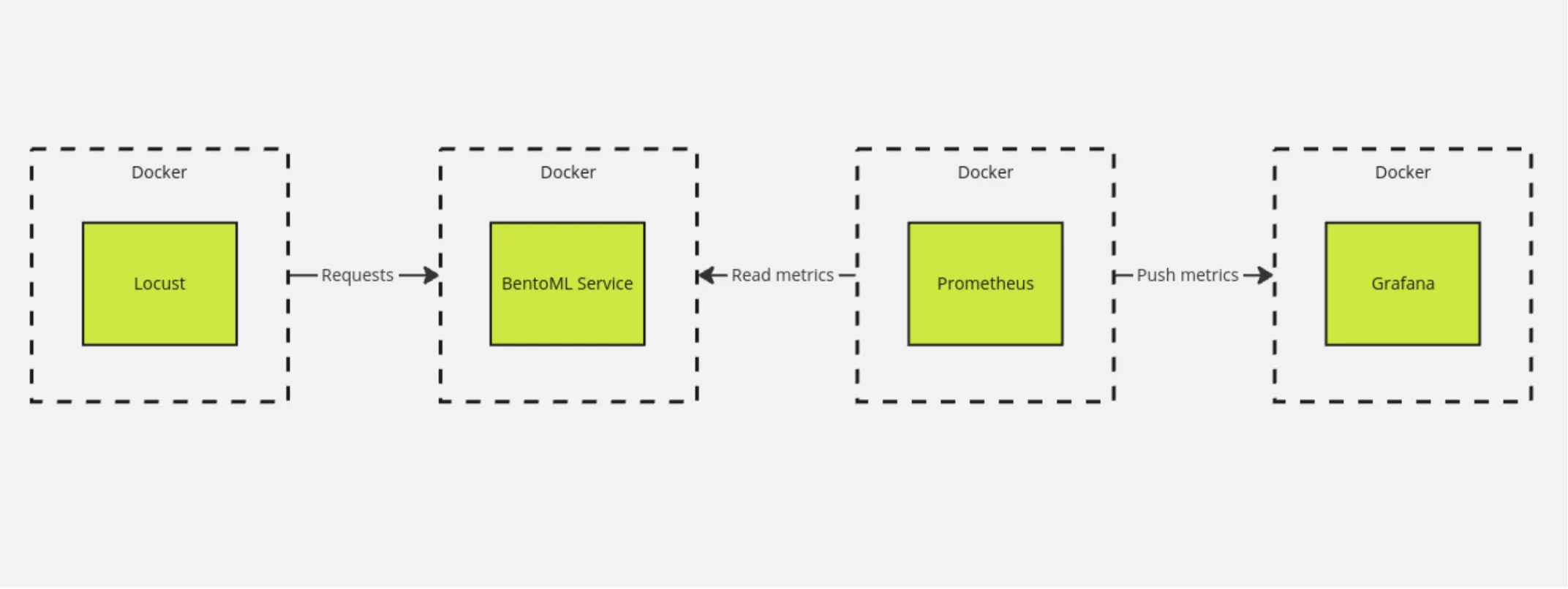
Architecture of the components in the scenario discussed.
How to do it?
We assume a machine learning model service is running locally and exposes a REST API. Here’s sample code that runs a model from the BentoML registry on port 3000:
bentoml serve <MODEL_NAME:TAG> -p 3000The docker-compose.yaml file below defines one locust service exposing port 8089, which talks to a service running locally on port 3000. The command run by the service relies on a Python script describing how the application should be tested. The command specifies how many users to simulate, how their number should grow over time, how long the simulation should run, and where to store the report and the file containing the simulation results.
version: '3'

services:
 locust:
   image: locustio/locust
   ports:
     - "8089:8089"
   volumes:
     - ./:/mnt/locust
   command: -f /mnt/locust/locustfile.py
   --host=http://host.docker.internal:3000 --headless --users 1000
   --spawn-rate 5 --run-time 5m --html /mnt/locust/results.html
   --csv /mnt/locust/results -t 5m
   extra_hosts:
     - "host.docker.internal:host-gateway"
Here’s what the options passed to the locust command mean (based on the documentation):
–host- the address where the ML service runs–headless- run without the graphical mode–users- the maximum number of users in the simulated traffic–spawn-rate- how many users get added to the current user pool in each given time interval–run-time- the overall duration of the simulation–html- the path where the HTML report will be stored--csv- the path where the CSV results will be stored
The extra_hosts section, together with a special address in the locust command, is needed so that the containerized tool can correctly reach a service running locally on the host machine (as described in this thread). If the ML model is available as a Docker container, every service required for the tests can be put into the docker-compose file.
The locustfile.py file holds an example of a single endpoint to be tested, along with a sample machine learning model payload.
from locust import HttpUser, between, task

EXAMPLE_DATA = {
   "data": ["This is an example sentence to classify."]
}

class QuickstartUser(HttpUser):
   """Load test user class."""

   wait_time = between(1, 5) # defines interval between user requests

   @task
   def classify(self):
       """Trigger `classify` endpoint."""
       self.client.post("/classify", json=EXAMPLE_DATA)
If docker-compose.yaml and locustfile.py sit in the same directory, simply run docker compose up to launch the container. Locust performs the simulation, and once it’s done, the results in .csv format and an HTML report are written to the current directory.
Reports
Running the load test produces an HTML report containing an interactive visualization of the service load, plus the results in .csv format.
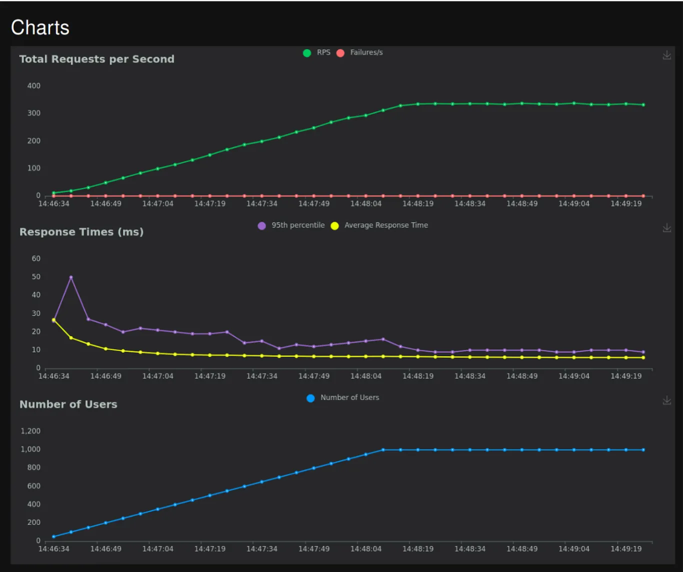
Charts of the user count, response time, and queries per second over the course of the traffic simulation.
The summary statistics with response times for every endpoint defined in locustfile.py. cover the 50th, 60th, 70th, 80th, 90th, 95th, 99th, and 100th percentiles of the model’s response time distribution. The values reported and used most often are the 95th and 99th percentile response times, which can be read as the longest response time to expect from the model in 95 or 99 percent of cases.
Monitoring system metrics
With Locust, we can observe, analyze, and report only on response time and on statistics of how the simulated requests were handled. Real-world machine learning models consume far more resources, GPUs included, and those are what we want to monitor and profile.
To do that, we can rely on Prometheus and Grafana to collect and visualize the logs emitted by our deployed ML model service.
At this point, if the model is deployed with the default metrics endpoint (/metrics), extra logs on system resource usage become available. To visualize them, we have to run Grafana, Prometheus, and a few other required services. For this, I’ll reuse an existing open-source docker-compose stack.
Below you’ll find the adjusted docker-compose.yaml file, which besides Grafana and Prometheus also launches the Locust container and kicks off load testing automatically.
version: '3.8'

volumes:
 prometheus_data: {}
 grafana_data: {}

services:
 locust:
   image: locustio/locust
   ports:
     - "8089:8089"
   volumes:
     - ./:/mnt/locust
   command: -f /mnt/locust/locustfile.py --host=http://host.docker.internal:8000
   --headless --users 100 --spawn-rate 5 --run-time 5m
   --html /mnt/locust/results.html --csv /mnt/locust/results -t 5m
   extra_hosts:
     - "host.docker.internal:host-gateway"
 prometheus:
   image: prom/prometheus
   restart: always
   volumes:
     - ./prometheus:/etc/prometheus/
     - prometheus_data:/prometheus
   command:
     - '--config.file=/etc/prometheus/prometheus.yml'
     - '--storage.tsdb.path=/prometheus'
     - '--web.console.libraries=/usr/share/prometheus/console_libraries'
     - '--web.console.templates=/usr/share/prometheus/consoles'
   ports:
     - 9090:9090
   extra_hosts:
     - "host.docker.internal:host-gateway"

 grafana:
   image: grafana/grafana
   user: '472'
   restart: always
   environment:
     GF_INSTALL_PLUGINS: 'grafana-clock-panel,grafana-simple-json-datasource'
   volumes:
     - grafana_data:/var/lib/grafana
     - ./grafana/provisioning/:/etc/grafana/provisioning/
   env_file:
     - ./grafana/config.monitoring
   ports:
     - 3000:3000
   depends_on:
     - prometheus
Let’s say the model runs locally on port 8000 with BentoML, started using the command:
bentoml serve handler.svc -p 8000.
Running docker compose up in the directory holding the docker-compose.yaml file starts all containers and kicks off load testing. Once Grafana is opened in the browser, the system metrics supplied by Prometheus are available. With a suitable dashboard, we can keep an eye on resource usage throughout load testing and the simulated network traffic.
It really is that easy! This set of application performance monitoring containers is generic and reusable. When you swap the model and update the BentoML handler, the only adjustment needed in the measurement setup is changing the endpoint name and sample data in the locustfile.py.
Results
The docker-compose.yaml we put together is a generic measurement setup for any model served over HTTP (BentoML is not a requirement), simulating the network traffic of users calling the ML service. Adding aggregation of system metrics additionally lets you track how the ML models consume key resources such as RAM, VRAM, CPU, and GPU. By tweaking the parameters of the simulated network traffic, you can run load tests, performance tests, and stress tests of ML services.
The screenshot below illustrates the tool in action. Throughout the simulation, GPU usage stays at a steady level, and scaling poses no risk of an Out Of Memory error. This way, we can test and confirm that our service is built so that growing traffic won’t break it.
System metrics visualized in Grafana.
Summary
This article showed how the Locust tool can simulate the load a service performing machine learning model inference will face. It presented simple code for testing exposed endpoints, the kinds of artifacts to expect, and how to make use of them. It also demonstrated how to visualize these metrics in Grafana, which comes in handy when designing ML service monitoring for production or during performance testing. I hope this article helps you design and analyze services and deployments involving machine learning models more effectively.