A Long Road – How the Machine Ends Up Interpreting Bytecode
An in-depth look at how the JVM interprets and compiles Java bytecode across several JIT compilation tiers, from the interpreter through the C1 and C2 compilers. Find out how these mechanisms boost application performance and efficiency.
I had heard before that the JIT (Just In Time) compiler is able to compile bytecode at several levels, but I never really considered what that means in practice. In mid-October, I attended a conference and had the chance to hear a talk on ‘lock-free programming’. In that talk, the speakers touched briefly on JVM internals, which made me want to explore the subject further. Since explaining something to others is one of the best ways to test whether you truly understand it, I decided to write this article.
Tiered compilation
A key difference between Java and languages such as C++ lies in how they are compiled. A C++ compiler turns code straight into machine code the CPU can run. Java, by contrast, compiles its code into an intermediate format called bytecode. The CPU can’t run this bytecode directly – it needs further processing. The JVM is the application that turns this bytecode into machine code so that the CPU can execute it.
Keep in mind that the code we write in any JVM-compatible language acts as a recipe describing how we want our program to run.
The JVM is able to compile our bytecode at five different levels. Here is an image that shows this:
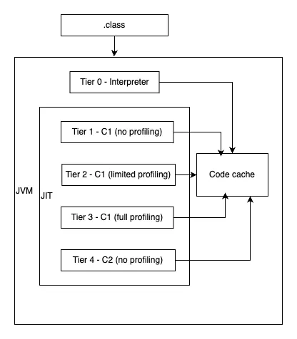
To show how the levels differ, I’ll use a very simple method as an example.
Bytecode (.class)
Here is the method defined in Java:
private static int resolveNumber(int i) {
    if (i < 20000) return i;
    else return i * 2;
}
Once it’s compiled, we can inspect the resulting bytecode with this command:
javap -c -p target/classes/org/zygiert/Main.class- javap is the Java Class File Disassembler shipped with the JDK.
- The -c option prints the disassembled code.
- The -v option makes private methods show up as well (this snippet is a fragment of the Main class).
The resulting bytecode is a sequence of JVM operation codes describing which operations should run. This is the method’s bytecode representation:
         0: iload_0
         1: sipush        20000
         4: if_icmpge     9
         7: iload_0
         8: ireturn
         9: iload_0
        10: iconst_2
        11: imul
        12: ireturn
This is what really happens:
iload_0puts an integer from a local variable onto the stack.sipushplaces the short integer20000on the stack.if_icmpgecompares the two integer values. When the first integer is greater than or equal to20000, it jumps to the instruction at byte offset 9. Otherwise, execution moves on to the next instruction.
When the integer is below 20000:
iload_0puts the parameter on the stack once more.ireturnreturns the integer from the stack.
When the integer is greater than or equal to 20000:
iload_0puts the parameter on the stack once more.iconst_2places the constant integer2on the stack.imulmultiplies the top two integers on the stack and leaves the product on the stack.ireturnreturns the resulting integer from the stack.
A quick clarification: the numbers on the left aren’t instruction numbers but byte offsets. For instance, the iload_0 instruction at byte offset 0 takes only 1 byte for its operation code. That’s why the sipush operation code comes right after it, at byte offset 1. The sipush instruction takes 3 bytes: 1 for the operation code and 2 more for the short integer it places on the stack. That’s why the if_icmpge operation code sits at byte offset 4.
These are only a handful of the available bytecode operation codes. The complete list is in the JVM specification. Remember, though, that this is just an intermediate representation of our code, which still has to be turned into machine code. That’s the interpreter’s job.
Interpreter
Today, the JVM relies on a template interpreter that converts every bytecode instruction into machine code at application startup. This happens each time the application is launched. Once the application starts, the template interpreter produces native code for every bytecode instruction, taking into account factors like the CPU architecture and the underlying operating system. The native code is then kept in the code cache.
To see how much time native code generation takes, run this command:
java -Xlog:startuptime -jar target/app.jar 10The printed log will contain a line like this one:
[0.019s][info][startuptime] Interpreter generation, 0.0014898 secsClearly, generating the interpreter is pretty fast.
From then on, the JVM has compiled native code tied to every bytecode instruction. So when a method runs in this state, the JVM walks through the bytecode and runs the matching native code for each instruction. This lets our application get going fairly fast, but it isn’t the most efficient approach.
To inspect the native code produced by the interpreter, run this command:
java -XX:+UnlockDiagnosticVMOptions -XX:+PrintInterpreter -jar target/app.jar 10The output is long, but every piece of native code is labelled with its operation code name, so finding what you need is easier. Here’s the iload_0 operation code as an example:
iload_0  26 iload_0  [0x000071666f9465e0, 0x000071666f946628]  72 bytes
[MachCode]
  0x000071666f9465e0: 4883 ec08 | c5fa 1104 | 24eb 1f48 | 83ec 10c5 | fb11 0424 | eb14 4883 | ec10 4889 | 0424 48c7
  0x000071666f946600: 4424 0800 | 0000 00eb | 0150 418b | 0641 0fb6 | 5d01 49ff | c549 ba80 | 1237 8666 | 7100 0041
  0x000071666f946620: ff24 da0f | 1f44 0000
[/MachCode]
It’s also worth noting that the JDK still contains a C++ interpreter, although modern JDK versions don’t use it by default.
C1 compiler
The C1 compiler, also called the client compiler, is part of the JIT compilation process. It kicks in when the JVM’s profiling mechanism notices that particular methods run frequently. The C1 compiler works at three different levels.
Tier 1
This tier is meant for trivial methods like getters, setters, or methods returning constant values. There’s nothing to gain from optimizing such methods further. No profiling data is collected at this tier, because none is needed.
Tier 2
At this level, the compiler relies on basic profiling information about the method. Because of this, the compiled method is smaller than one compiled at Tier 3. Usually, once the JVM notices that a method is hot, it compiles it to Tier 3 and afterwards to Tier 4.
It’s worth explaining what makes a method hot. There are two ways a method can become hot:
- The number of its invocations goes above
TierXInvocationThresholdmultiplied byCompileThresholdScaling. - The number of its invocations goes above
TierXMinInvocationThresholdmultiplied byCompileThresholdScaling, and its invocation count plus the number of loop iterations inside it goes aboveTierXCompileThresholdmultiplied byCompileThresholdScaling.
If the Tier 4 compilation queue is too long, however, waiting may not pay off. On top of that, leaving a method compiled at Tier 3 can be wasteful because of the extra size and complexity that come with the additional profiling data. In these situations, the method may get recompiled to Tier 2, and later it may be compiled to Tier 3 again and then to Tier 4.
Tier 3
Once a method is recognized as hot, it’s typically compiled to Tier 3, which carries full profiling data. This Tier is often just an intermediate step on the way to Tier 4. As noted above, though, in some cases the method may end up compiled to Tier 2 rather than moving straight on to Tier 4.
Inspecting compiled code details
Earlier, I said that methods compiled by the C1 compiler vary in size and in how much profiling data they get. Let’s now see this in practice.
To make the JVM stop compiling at a given Tier and print information about method compilation, you can target the C1 Tier with this command:
java -XX:+PrintCompilation -XX:TieredStopAtLevel=1 -jar target/app.jar 15000-XX:+PrintCompilationturns on printing of compilation details.-XX:TieredStopAtLevel=1tells the JVM to stop compiling at Tier 1.
Among the methods listed, you’ll see the resolveNumber method:
46 20 1 org.zygiert.Main::resolveNumber (13 bytes)46is the time in milliseconds since the program was started.20is the compilation ID.1is the compilation Tier.org.zygiert.Main::resolveNumberis the method signature.(13 bytes)shows the size of the bytecode.
Now that we’ve made the C1 compiler compile our method to Tier 1, the next step is to look at the native code actually produced for it, plus a few extra details. For that, I’ll use two JVM options:
-XX:+UnlockDiagnosticVMOptions, which enables JVM diagnostic options.-XX:+PrintAssembly, which prints the native code.
Here is the complete command:
java -XX:+UnlockDiagnosticVMOptions -XX:+PrintAssembly -XX:TieredStopAtLevel=1 -jar target/app.jar 15000The output is large, but you can find the resolveNumber method in it. This is what the beginning of the printed details looks like:
Compiled method (c1) 122   20       1       org.zygiert.Main::resolveNumber (13 bytes)
 total in heap  [0x0000719a289a3888,0x0000719a289a3a60] = 472
 main code      [0x0000719a289a3980,0x0000719a289a3a28] = 168
 stub code      [0x0000719a289a3a28,0x0000719a289a3a58] = 48
 oops           [0x0000719a289a3a58,0x0000719a289a3a60] = 8
 mutable data [0x00007199d8024530,0x00007199d8024568] = 56
 relocation     [0x00007199d8024530,0x00007199d8024560] = 48
 metadata       [0x00007199d8024560,0x00007199d8024568] = 8
 immutable data [0x00007199d80244b0,0x00007199d8024520] = 112
 dependencies   [0x00007199d80244b0,0x00007199d80244b8] = 8
 scopes pcs     [0x00007199d80244b8,0x00007199d8024508] = 80
 scopes data    [0x00007199d8024508,0x00007199d8024520] = 24
What interests me most right now is total in heap. The property’s name can be misleading, but it really shows how much code cache memory this compiled method takes up. Here, the total size is 472 bytes, whereas the method’s actual implementation takes 168 bytes.
We can then do the same for Tier 2 and Tier 3. I’ll skip the output, but here are the sizes for each tier.
| Tier 1 | Tier 2 | Tier 3 | |
|---|---|---|---|
| overall size | 472 | 536 | 576 |
| size of main code | 168 | 232 | 272 |
These numbers show why a method that can’t be compiled from Tier 3 to Tier 4 falls back to Tier 2. Thanks to the limited profiling data, it’s smaller.
C2 compiler
This is the last compilation stage, where hot methods end up. It’s frequently called the server compiler, and it applies a number of aggressive optimizations such as branch prediction, vectorization, and loop unrolling.
Many of these optimizations are based on predictions. In other words, using profiling data, the JVM assumes that a method will run the same way it did before. That assumption doesn’t always hold, though. When it doesn’t, the JVM notices the mismatch and falls back to interpreted code for that method. Profiling data for the method is then collected anew, and the whole compilation cycle may start over.
As noted before, methods compiled by C2 are heavily optimized and carry no profiling data. To see the details, run this command:
java -XX:+UnlockDiagnosticVMOptions -XX:+PrintAssembly -XX:-BackgroundCompilation -jar target/app.jar 15000This command adds the option:
-XX:-BackgroundCompilation, which makes the JIT compiler compile methods synchronously instead of in the background. I needed this option because my program ends very quickly, and without it the compilation might not finish before the program exits.
With that, we can expand the earlier table with the C2-compiled version of the resolveNumber method.
| Tier 1 | Tier 2 | Tier 3 | Tier 4 | |
|---|---|---|---|---|
| overall size | 472 | 536 | 576 | 392 |
| size of main code | 168 | 232 | 272 | 112 |
C2 compilation yields the smallest compiled method, which shows that C2 brings real benefits even for simple methods. Its main downside, however, is that it costs time and resources.
Note that the -XX:CICompilerCount option lets us control how many threads the JIT compiler uses. There’s also an option called -XX:CICompilerCountPerCPU. When it’s turned on, the JVM decides automatically how many JIT compiler threads to use based on the number of available CPU cores. For example, on a 4-core CPU you can expect 2 threads for the C2 compiler and 1 thread for the C1 compiler.
Several options also exist for controlling the thresholds of each compilation tier. I won’t describe them in detail, but you can list them with this command:
java -XX:+PrintFlagsFinal | grep TierCode cache
There’s one more piece I’d like to cover: the code cache. After code is compiled, it has to be kept somewhere easy to reach. By default, the code cache is split into three segments:
- JVM internal (non-method) code – this segment holds interpreted code, which stays in the cache permanently. Its size can be set with the
-XX:NonProfiledCodeHeapSizeoption. - Profiled-code – this segment contains lightly optimized code produced by the C1 compiler and is short-lived. Its size can be set with the
-XX:ProfiledCodeHeapSizeoption. - Non-profiled code – this segment holds fully optimized code produced by the C2 compiler. Its size can be controlled with the
-XX:NonNMethodCodeHeapSizeoption.
There are also a few other code cache-related JVM options that may come in handy:
-XX:InitialCodeCacheSize-XX:ReservedCodeCacheSize-XX:CodeCacheExpansionSize-XX:+PrintCodeCache
Conclusion
My goal in this blog post was to explain the core concepts behind turning bytecode into native code. The process is very dynamic and highly configurable. It does take considerable time and resources, but over time it can greatly improve the performance of our programs.
Every example in this article was run on Ubuntu 24.04.3 LTS, x86_64, with OpenJDK Runtime Environment Temurin-25+36 (build 25+36-LTS). I hope this article gives you a clearer picture of how the JVM produces native code.