Triton Inference Server: Tips and Tricks
A cheat sheet of handy Triton commands and configurations to come back to whenever you work with this tool.
This is my second post about Triton Inference Server. The first one covered its features and use cases. If you haven’t read it and some concepts in this text are unclear to you, I recommend going through it first.
In this post, you’ll find tips and tricks, a cheat sheet of handy commands, and code samples for benchmarking various configurations of computer vision models. It is more technical than the previous one: after reading it, you’ll know concrete commands for optimizing and configuring models served by Triton.
Note: all the commands below use containers in versions 22.04 or 22.11, but feel free to pick any version that suits you. These containers depend on CUDA drivers, so the versions I use below may not work in your environment.
Cheatsheets
- Running Triton in a docker container
Important note: You need to pass the absolute path of the current directory and mount it under the same path in the container filesystem. If you don’t, Triton won’t find the models in the model-repository
-
Using the model-analyzer tool in a docker container
-
Defining a global response cache
Defining a model response cache
-
in config.pbtxt:
-
Defining the models poll interval
-
A typical model-repository structure
-
Defining dynamic batching (here, 100 microseconds is the time used to aggregate a dynamic batch)
in config.pbtxt: -
Defining the model’s max batch size (here, the maximum batch size is 8)
in config.pbtxt: -
Model warmup
Put this line in config.pbtxt. The key field has to match the name, type, and dims of the defined input.
-
TensorRT optimization (using a half-precision model and defining the max workspace size)
-
OpenVINO optimization (for models running on CPU)
-
TF JIT optimization
-
TensorFlow XLA optimizations
-
TensorFlow with automatic FP16 optimization
Tips & tricks - what I wish I had known before experimenting with Triton
-
When using model-analyzer in a docker container, remember to mount the volume containing model-repository under the same path in the container as on the host filesystem. If you don’t, model-analyzer will have trouble locating the deployed models:
-
Exporting the model to TensorRT is done with this docker image:
Because of version validation, it’s crucial that the tensorrt container has the same version as tritonserver. Put differently, Triton won’t serve a model exported with another TensorRT version.
-
A basic command for converting an ONNX model to TensorRT:
-
To export the model in half-precision, You can add these flags:
On MobileNetV3, this optimization brought up to a 2x speedup in latency and throughput compared to the FP32 ONNX model.
- To export the model in a quantized format (with some weights stored as int8), use these flags:
On MobileNetV3, this optimization brought up to a 2-3x speedup in latency and throughput compared to the FP32 ONNX model.
- Exporting the model with a dynamic batch size requires passing 3 parameters to the trtexec program. For a model trained on ImageNet, they may look like this:
On MobileNetV3, this optimization brought up to a 2x speedup in latency and throughput compared to models running in single batch mode.
- To get higher throughput and lower latency in single batch mode, You should use an explicit batch size.
The model with an explicit batch size achieved roughly 20% higher throughput and 16% shorter inference time than the model with a dynamic batch size.
- When exporting a model to ONNX (e.g. from PyTorch code) with a dynamic batch size, You need to set the _dynamicaxes parameter:
Defining input and output names gives you more control over parameter names at inference time. If you skip this, names derived from the model’s layer names are used.
To understand the process better, have a look at the PyTorch example.
- config.pbtxt:
Set the model’s _max_batchsize to a sensible value greater than or equal to 1. If the model doesn’t support dynamic batches – for instance, a model exported to TensorRT with an explicit batch size of 1 – You should set this value to 1.
When _max_batchsize is greater than 1, the first dimension in _dims _is always -1 by default. If You define dims: [3, 224, 224], Triton will prepend -1 to the list for You.
- model-analyzer:
When You run model analysis and tune Triton configuration parameters in a docker container, remember to mount the volume with the model-repository inside the container under the same path as on the host machine. If you don’t, _perfanalyzer and _modelanalyzer will have a hard time finding the models.
The documentation and the full list of parameters of the _modelanalyzer are available here.
-
A sample command:
-
_perfanalyzer:
Analyzing models that work on images is tricky when You can’t send random data in requests. In that case, You can prepare a file containing sample data to send in a request. The file follows a predefined format, with the data as a flat list of values and the shape of the target tensor. In the example below, I want to send an image with shape (640, 480, 3), yet in the “content” field I need to provide the image as a flat list of values – here, with shape (921600,).
-
A command using sample data stored in a
data.jsonfile looks like this: -
Ensemble model
To satisfy Triton’s requirements, You need to create an empty directory with a version.
Ensemble model
As an example, here is how deploying a ViT model as a Python model looks:
Triton requires the initialize and execute functions. During initialization, the model and the feature extractor are loaded from huggingface. execute performs some preprocessing, invokes the models, and returns the results.
Its config.pbtxt:
And the directory looks as follows:
Next, I show You the ViT model deployed as an ensemble model, with pre- and post-processing separated out.
_ensemblemodel/config.pbtxt:
preprocessing/1/model.py:
preprocessing/config.pbtxt:
vit/config.pbtxt:
The directory structure looks as follows:
Compare these two deployment configurations. It’s clear that optimizing the core model speeds up the inference pipeline by up to roughly 30%.
Benchmark code
For the benchmark, I picked MobileNetV2. Below, You’ll find two tables with results for various batch sizes.
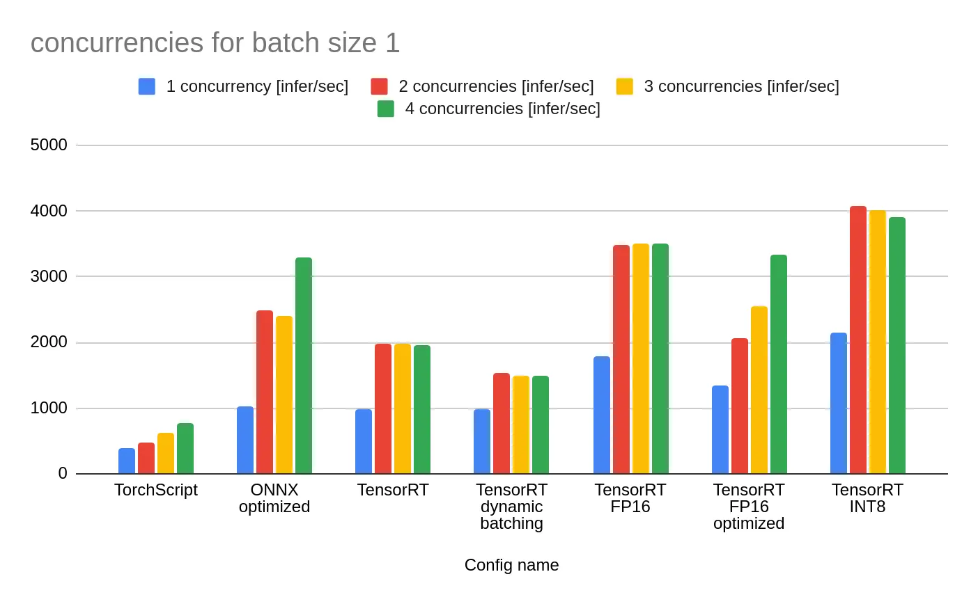
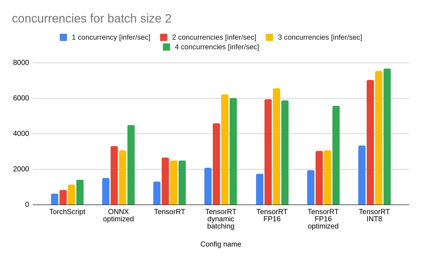
Unsurprisingly, TorchScript with no optimizations performs worst in this comparison. The table above shows that raising _batchsize with dynamic batching leads to higher throughput. Converting the model to FP16 and INT8 yields a noticeable speedup, though it may lower the model’s performance. Interestingly, TensorRT FP16 achieves higher throughput than TensorRT FP16 optimized. The former was exported as a half-precision model, while the latter was exported in full precision and configured in Triton to run in FP16. The chart above suggests that if you want a half-precision model, it’s better to export it in that form rather than rely on Triton’s conversion. As always, results vary across hardware, so you should test every configuration on Your machine before deploying.
Summary
This post offers a cheat sheet of handy Triton commands and configurations to come back to whenever you work with this tool. It includes code and benchmarks for various configurations of a computer vision model. The reader followed the process of optimizing a complex model by splitting the pre- and post-processing code from the model inference itself. I hope you picked up something new today, and I encourage you to experiment with Triton. I suspect the two of you might get along 🙂